Basic Notions
Methods:
- Inverse Function
- Acceptance-Rejection
- Composition
- Convolution
- Transformations
Distributions:
- Uniform
- General Discrete
- Geometric
- Poisson
- Exponential
- Pareto
- Normal
- Gamma
- Beta
Cross Referencing:
- Topics Index
- SimSpiders Main Page
|
General Discrete Distribution
The Inverse Function Method:
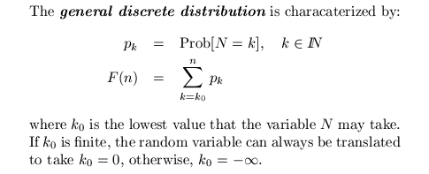
Suppose that k0=0. The
Inverse Function Method then requires
setting N(U) = min{k : F(k+1) > U}.
- Generate U~U(0,1)
- F(0) = p0, k = 0.
- While (F(k) < U)
- k = k+1, F(k) = F(k-1) + pk
- Set N = k
Notice that the
average number of iterations
will always be E[N] + 1 when the above algorithm is used. This is so because
the number of times that the algorithm passes through the while
operation is precisely N+1, where N is the final value.
Accelerating Techniques: Buckets
The Method of Buckets combines the
Composition and the
Inverse Function methods
for generating random variables and works well especially when generating
empirical discrete distributions with a large number of values. See Bratley,
Fox and Sxrhage (**reference). A total of M
buckets are defined by the subintervals
[m/M, (m+1)/M) for m=0, ..., M-1. The m-th bucket is composed of
all those indices k such that F(k) lies within [m/M, (m+1)/M) plus the
last element. Call b(m) the first element of the m-th bucket.

|
The figure shows the bucket B2 containing elements {1,2,3}. when
we generate a random variable U, instead of searching as in the previous
algorithm, we now narrow the search by looking for the bucket and then
finiding the value within the bucket.
- Generate U~U(0,1)
- Bucket m = Integer value of (M U), set k = b(m).
- While (F(k) < U)
- k = k+1, F(k) = F(k-1) + pk
- Set N = k
The average number of iterations now can be calculated by conditioning on $U$
belonging to the intervals of the form [m/M, (m+1)/M). Given the
bucket m, N = X(m) + b(m) where X(m) has the corresponding residual
distribution. Clearly, E[X(m)] &\lt; E[N] and equality only hapens if all the
elements belong to the last bucket, for only then will b(m) = 0 for all m.
Buckets are equally probable and the number of iterations required given
bucket m is E[X(m)] + 1. Therefore a reduction in computational time can be
achieved.
|
Accelerating Techniques: Memory vs Speed
If the random variable N has a finite number of values, it may be more
advantageous to calculte the distribution F(k) and keep it in memory, rather
than evaluating F(k) = F(k-1) + pk every time we want to generate
a random variable.
|
Accelerating Techniques: Reordering
The order in which the comparisons are made in the algorithm above
is always the same, starting with
k=0 and going upwards. Suppose that a particular value, say k=5 has a much
larger probability than other values. If the inverse funtion method above is
used, then most of the time at least five comparisons or iterations of the
algorithms have to be made. Instead, we may reorder the values by
decreasing probability.
A correspondence between two random variables is established, setting a
unique function X(N) that assigns to the value N its order, so that X(N) = 0
for the value of N with highest probability, X(N)=k for the (k+1)-st most
probable value. The random variable X is then generate by the Inverse Method
above, and N is set to the unique corresponding value. The average
number of
iterations is now E[X]+1 < E[N] +1.
|

|
|


